网络安全研究人员提出了一种新颖的方法，该方法利用来自物联网 (IoT) 设备的电磁场发射作为旁道来收集有关针对嵌入式系统的不同类型恶意软件的精确知识，即使在应用了混淆技术的场景中也可检测出来。

随着物联网设备的快速普及，为威胁参与者提供了一个有吸引力的攻击面，部分原因是它们配备了更高的处理能力并能够运行功能齐全的操作系统，最新研究旨在改进恶意软件分析以减轻潜在的安全风险。

研究结果由计算机科学与随机系统研究所 (IRISA) 的一组学者在上个月举行的年度计算机安全应用会议 ( ACSAC ) 上公布。

研究人员在一篇论文中说： “从设备测量的[电磁]辐射实际上无法被恶意软件检测到。” “因此，与动态软件监控不同，恶意软件规避技术不能直接应用。此外，由于恶意软件无法控制外部硬件级别，因此无法关闭依赖硬件功能的保护系统，即使恶意软件拥有机器上的最大权限。”

目标是利用侧信道信息检测与之前观察到的模式不同的发射异常，并在与系统正常状态相比记录模拟恶意软件的可疑行为时发出警报。

这不仅不需要对目标设备进行修改，研究中设计的框架还可以检测和分类隐蔽恶意软件，例如内核级 rootkit、勒索软件和分布式拒绝服务 (DDoS) 僵尸网络，例如 Mirai，以及数以看不见的变种。

侧信道方法分三个阶段进行，包括在执行 30 种不同的恶意软件二进制文件时测量电磁辐射，以及执行与视频、音乐、图片和相机相关的良性活动，以训练卷积神经网络 ( CNN ) 模型以对真实数据进行分类。世界恶意软件样本。具体来说，该框架将可执行文件作为输入，并仅依靠侧信道信息输出其恶意软件标签。

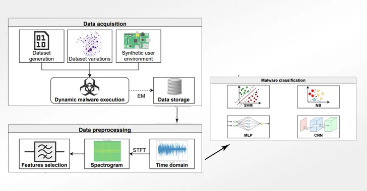
在实验设置中，研究人员选择 Raspberry Pi 2B 作为具有 900 MHz 四核 ARM Cortex A7 处理器和 1 GB 内存的目标设备，使用示波器和 PA 303 BNC 的组合采集和放大电磁信号前置放大器，有效预测三种恶意软件类型及其相关家族，准确率分别为 99.82% 和 99.61%。

研究人员总结道：“[B] 使用简单的神经网络模型，可以通过仅观察其 [电磁] 辐射来获得有关受监控设备状态的大量信息。” “我们的系统可以抵御各种代码转换/混淆，包括随机垃圾插入、打包和虚拟化，即使系统以前不知道这种转换。”

论文详情

https://dl.acm.org/doi/10.1145/3485832.3485894

物联网 (IoT) 由数量和复杂性呈指数增长的设备组成。他们使用大量定制的固件和硬件，而没有考虑安全问题，这使他们成为网络犯罪分子，尤其是恶意软件作者的目标。

我们将介绍一种使用侧信道信息来识别针对设备的威胁类型的新方法。使用我们的方法，即使存在可能阻止静态或符号二进制分析的混淆技术，恶意软件分析师也能够获得有关恶意软件类型和身份的精确知识。我们从被各种野外恶意软件样本和真实的良性活动感染的物联网设备中记录了 100,000 条测量轨迹。我们的方法不需要对目标设备进行任何修改。因此，它可以独立于可用资源进行部署，而无需任何开销。此外，我们的方法的优点是恶意软件作者很难检测到和规避它。在我们的实验中，我们能够以 99.82% 的准确率预测三种通用恶意软件类型（和一种良性类别）。。更重要的是，我们的结果表明，我们能够在训练阶段使用看不见的混淆技术对更改的恶意软件样本进行分类，并确定对二进制文件应用了哪种混淆，这使得我们的方法对恶意软件分析人员特别有用。

项目地址

GitHub

https://github.com/ahma-hub/analysis/wiki

该存储库包含 ACSAC 2021 中发表的论文 Obfuscation Revealed: Leveraging Electromagnetic Signals for Obfuscated Malware Classification 的代码、数据集和模型文档。

恶意软件和良性数据集

要求

该数据集包含为恶意软件和良性数据集编译的 ARM 可执行文件。可执行文件在 Linux raspberrypi 4.19.57-v7+ ARM 上编译。

用法

所有可执行文件都可以直接在目标设备上执行。该数据集分为 5 个不同的系列：bashlite、gongcry、mirai、rootkit、goodware。除了需要安装的rootkits如下：

Keysniffer Rootkit

Rootkit 安装：

sudo insmod kisni-4.19.57-v7+.ko

对于 rootkit 卸载：

sudo rmmod kisni-4.19.57-v7+.ko

MaK_It rookit

每次目标设备重启只运行一次：

ARG1=".maK_it"
ARG2="33"
rm -f /dev/$ARG1 #确保其干净
echo "Creating virtual device /dev/$ARG1"
mknod /dev/$ARG1 c $ARG2 0
chmod 777 /dev/$ARG1
echo "Keys will be logged to virtual device."

对于 rootkit 卸载：

echo "debug" > /dev/.maK_it ; echo "modReveal" > /dev/.maK_it; #Un-hide rookit
sudo rmmod maK_it4.19.57-v7+.ko; #Uninstall rootkit

对于 rootkit 安装：

sudo insmod maK_it4.19.57-v7+.ko

有关在目标设备上执行恶意软件的命令的详细信息，请参阅子文件夹 cmdFiles

注意：此存储库是为研究目的而制作的。对于因您访问此存储库或以任何其他方式使用此存储库而在您的计算机、软件、设备或其他财产上安装病毒或恶意软件而造成的任何损害，我们概不负责。

数据采集

当前存储库包含与论文中发布的数据采集接口交互所需的所有脚本：“混淆揭示：电磁混淆恶意软件分类”。

要求

此存储库支持 PicoScope® 6000 系列示波器。要安装所需的 Python 包：

pip install -r requirements.txt

数据采集设置

目标设备

我们在设置中使用 Raspberry Pi (1,2,3)。它通过 SSH 通过以太网连接到主机分析机。SSH IP 配置可以在generate_traces_pico.py .

ssh.connect('192.168.1.177', username='pi')

示波器、放大器和探头

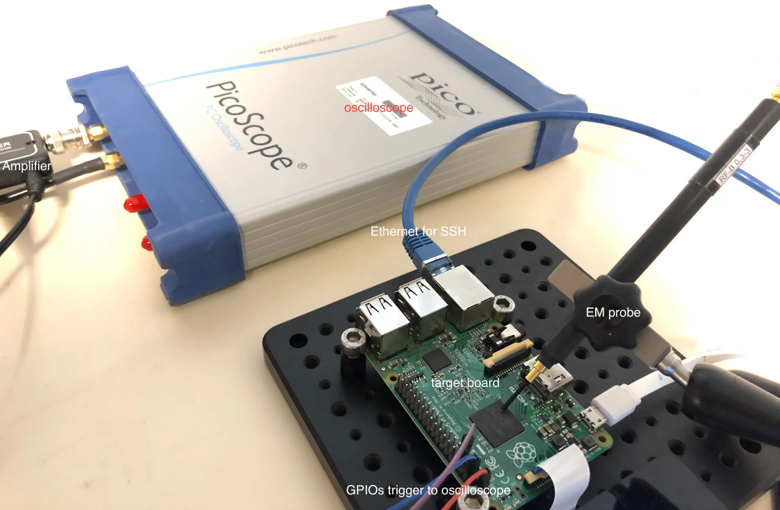
我们使用 Langer PA-303 +30dB 作为放大器，连接到 H-Field Probe (Langer RF-R 0.3-3) 和 Picoscope 6407 1GHz 带宽。探头通过放大器连接到端口 A，而来自目标设备的触发器连接到 Picoscope 的端口 B。

包装器配置

为了触发示波器，我们在设备上启动了一个包装程序。这个包装器将简单地发送触发器并在相应的时间启动我们想要监视的程序。它由 generate_traces_pico.py 自动调用。您只需要精确其在受监控设备上的路径即可。编译后的包装器可以存储/home/pi/wrapper在generate_traces_pico.py . 封装器已经配置了 Raspberry Pi Plug P1 引脚 11，即 GPIO 引脚 17，作为示波器的触发输入。

命令文件

您现在需要在类似 CSV 的文件 cmdFile 中提供要监视的命令列表。

该文件必须采用以下形式：pretrigger-command,command,tag对于 cmdFile 的每一行，每次循环迭代都将执行以下操作：

pretrigger command通过 SSH 在设备上执行
武装示波器
触发示波器并执行被监控的 command
将数据记录在一个名为 tag-$randomId.dat

用于启动密钥嗅探器的命令文件示例：

sudo rmmod kisni,./keyemu/emu.sh A 10,keyemu
sudo insmod keysniffer/kisni-4.19.57-v7+.ko,./keyemu/emu.sh A 10,keyemu_kisni

启动进程跟踪捕获

跟踪捕获示例：

./generate_traces_pico.py ./cmdFiles/cmdFile_bashlite.csv -c 3000 -d ./bashlite-2.43s-2Mss/ -t B --timebase 80 -n 5000000

这将从示波器捕获 3000 条跟踪，使用 cmdFile_bashlite.csv 中定义的路径在目标设备上执行 Bashlite 恶意软件，并将跟踪输出到./bashlite-2.43s-2Mss主机分析机器上的文件夹。示波器将以块模式执行，采样频率为“80”。有关更多详细信息，请参阅data-acquisition存储库。

预训练模型

该存储库包含每个场景以及每个深度学习 (DL) 和机器学习 (ML) 算法的所有预训练模型。深度学习模型以 7z 格式压缩，它们需要解压缩才能与其他模块一起使用，run_decompression.sh用于解压缩文件。

分析工具

测试数据集的验证

要求

为了能够运行分析，您（可能）需要 python 3.6 和所需的包：

pip install -r requirements.txt

测试数据集

有两个数据集可用于在以下网站上重现结果

https://zenodo.org/record/5414107

这两个数据集是：

traces_selected_bandwidth.zip: 从测试数据集中提取的频谱图带宽 (40)，以重现论文中提出的分类结果，
raw_data_reduced_dataset.zip: 一组减少的原始电磁迹线，用于重现端到端过程（预处理和分类）。

测试数据集的评估

初始化

为了更新数据的位置，您之前下载了需要运行脚本的列表update_lists.sh：

./update_lists  [存储列表的目录] [存储(下载的)跟踪目录]

这必须应用于目录list_selected_bandwidth并list_reduced_dataset 分别与数据集相关联：traces_selected_bandwidth.zip和raw_data_reduced_dataset.zip

例如：

./update_lists  ./lists_selected_bandwidth/ ./traces_selected_bandwidth

机器学习 (ML) 评估

要运行所有机器学习实验的计算，您可以使用脚本run_ml_on_reduced_dataset.sh和run_ml_on_extracted_bandwidth.sh：

./run_ml_on_extracted_bandwidth.sh  [directory where the lists are stored] [directory where the models are stored] [directory where the accumulated data is stored (precomputed in pretrained_models/ACC) ]

结果存储在文件中ml_analysis/log-evaluation_selected_bandwidth.txt。模型和累加器在名为的存储库中可用pretrained_models。

例如：

./run_ml_on_extracted_bandwidth.sh lists_selected_bandwidth/ ../pretrained_models/ ../pretrained_models/ACC

./run_ml_on_reduced_dataset.sh

结果存储在文件中ml_analysis/log-evaluation_reduced_dataset.txt。

深度学习 (DL) 评估

要使用预训练模型在测试数据集上运行所有深度学习实验的计算，您可以使用脚本run_dl_on_selected_bandwidth.sh：

./run_dl_on_selected_bandwidth.sh  [directory where the lists are stored] [parent directory where the models are stored with subdirectories MLP/ and CNN/ (precomputed in pretrained_models/{CNN and MLP})] [directory where the accumulated data is stored (precomputed in pretrained_models/ACC) ]

结果存储在文件中evaluation_log_DL.txt。

例如：

./run_dl_on_selected_bandwidth.sh ../lists_selected_bandwidth/ ../pretrained_models/ ../pre-acc/

要使用缩减数据集（从 zenodo 下载）为 MLP 和 CNN 架构训练和存储预训练模型，您可以使用脚本run_dl_on_reduced_dataset.sh：

./run_dl_on_reduced_dataset.sh  [directory where the lists are stored] [directory where the accumulated data is stored (precomputed in pretrained_models/ACC) ] [DL architecture {cnn or mlp}] [number of epochs (e.g. 100)] [batch size (e.g. 100)]

模型以h5-files 的形式存储在与分类方案名称相同的目录中。所有场景和带宽的验证精度都存储在training_log_reduced_dataset_{mlp,cnn}.txt.

“提取的带宽”数据集的结果


场景	#	MLP AC [ ${\epsilon}_{opt}$ ]	CNN AC [ ${\epsilon}_{opt}$ ]	LDA + NB AC [ ${\epsilon}_{opt}$ ]	LDA + NB AC [ ${\epsilon}_{opt}$ ]
类型	4	99.75% [28]	99.82% [28]	97.97% [22]	98.07% [22]
家族	2	98.57% [28]	99.61% [28]	97.19% [28]	97.27% [28]
虚拟化	2	95.60% [20]	95.83% [24]	91.29% [6]	91.25% [6]
封隔器	2	93.39% [28]	94.96% [20]	83.62% [16]	83.58% [16]
混淆	7	73.79% [28]	82.70% [24]	64.29% [10]	64.47% [10]
可执行	35	73.56% [24]	82.28% [24]	70.92% [28]	71.84% [28]
Novelty (familly)	5	88.41% [16]	98.85% [24]	98.25% [6]	98.61% [10]

脚本下载地址

①GitHub

https://github.com/ahma-hub.zip

②云中转网盘:

https://yzzpan.com/#sharefile=ACR5vmS7_25988
解压密码:www.ddosi.org

脚本概述及列表

.
├── README.md
├── requirements.txt
│── run_dl_on_selected_bandwidth.sh #> script to run the DL for all scenarii on  
|                                   # the (full) testing dataset (available on zenodo) 
|                                   # using pre-computed models
|── run_dl_on_reduced_dataset.sh    #> script to run the training on 
|                                   # on a reduced dataset (350 per samples per 
|                                   # executable, available on zenodo)
│── run_ml_on_reduced_dataset.sh    #> script to run the end-to-end analysis on 
|                                   # on a reduced dataset (350 per samples per 
|                                   # executable, available on zenodo)
│── run_ml_on_selected_bandwidth.sh #> script to run the ML classification for all
|                                   # for all scenarii on the testing pre-computed 
|                                   # dataset (available on zenodo)
│── update_lists.sh                 #> script to update the location of the traces 
│                                   # in the lists 
│
├── ml_analysis
│   │── evaluate.py                            #> code for the LDA + {NB, SVM} on the 
|   |                                          # reduced dataset (raw_data_reduced_dataset)
|   |── NB.py                                  #> Naïve Bayensian with known model 
|   |                                          # (traces_selected_bandwidth)
|   |── SVM.py                                 #> Support vector machine with known model
|   |                                          # (traces_selected_bandwidth)
│   │── log-evaluation_reduced_dataset.txt     #> output log file for the ML evaluation
|   |                                          # on the reduce datasete
│   │── log-evaluation_selected_bandwidth.txt  #> output log file for the ML evaluation
|                                              # using the precomputed models
│ 
│
│
├── dl_analysis
│   │── evaluate.py            			#> code to predict MLP and CNN using pretrained models
│   │── training.py            			#> code to train MLP and CNN and store models 
|   |                          			# according to best validation accuracy   
│   │── evaluation_log_DL.txt  			#> output log file with stored accuracies on the testing dataset
|   |── training_log_reduced_dataset_mlp.txt    #> output log file with stored validation accuracies 
|   |                          			# on the reduced dataset for the mlp neural network over all scenarios and bandwidths
|   |── training_log_reduced_dataset_cnn.txt    #> output log file with stored validation accuracies 
|   |                          			# on the reduced dataset for the cnn neural network over all scenarios and bandwidths
|
│
│
├── list_selected_bandwidth    #> list of the files used for training, 
│   │                          # validating and testing (all in one file)
│   │                          # for each sceanario (but only the testing 
|   |                          # data are available). Lists associated to
|   |                          # the selected bandwidth dataset
│   │── files_lists_tagmap=executable_classification.npy                              
│   │── files_lists_tagmap=novelty_classification.npy   
│   │── files_lists_tagmap=packer_identification.npy
│   │── files_lists_tagmap=virtualization_identification.npy
│   │── files_lists_tagmap=family_classification.npy 
│   │── files_lists_tagmap=obfuscation_classification.npy
│   │── files_lists_tagmap=type_classification.npy   
│
│
├── list_reduced_dataset    #> list of the files used for training, 
│   │                       # validating and testing (all in one file)
│   │                       # for each sceanario. Lists associated to
|   |                       # the reduced dataset
│   │── files_lists_tagmap=executable_classification.npy                              
│   │── files_lists_tagmap=novelty_classification.npy   
│   │── files_lists_tagmap=packer_identification.npy
│   │── files_lists_tagmap=virtualization_identification.npy
│   │── files_lists_tagmap=family_classification.npy 
│   │── files_lists_tagmap=obfuscation_classification.npy
│   │── files_lists_tagmap=type_classification.npy   
│
├── pre-processings            #> codes use to preprocess the raw traces to be 
    │                          # able to run the evaluations
    │── list_manipulation.py   #> split traces in {learning, testing, validating} 
    │                          # sets 
    │── accumulator.py         #> compute the sum and the square of the sum (to 
    │                          # be able to recompute quickly the NICVS)  
    │── nicv.py                #> to compute the NICVs
    │── corr.py                #> to compute Pearson coeff (alternative to the 
    |                          # NICV)
    │── displayer.py           #> use to display NICVs, correlations, traces...
    │── signal_processing.py   #> some signal processings (stft, ...)
    |── bandwidth_extractor.py #> extract bandwidth, based on NICVs results
    |                          # and creat new dataset
    │── tagmaps                #> all tagmaps use for to labelize the data 
        │                      # (use to creat the lists)
    	│── executable_classification.csv  
    	│── family_classification.csv
    	│── novelties_classification.csv  
    	│── obfuscation_classification.csv  
    	│── packer_identification.csv  
    	│── type_classification.csv  
    	│── virtualization_identification.csv

evaluate.py用法

usage: evaluate.py [-h] 
                   [--lists PATH_LISTS]  
                   [--mean_size MEAN_SIZES]  
                   [--log-file LOG_FILE]  
                   [--acc PATH_ACC]  
                   [--nb_of_bandwidth NB_OF_BANDWIDTH]  
                   [--time_limit TIME_LIMIT]  
                   [--metric METRIC]

optional arguments:
  -h, --help                         show this help message and exit
  --lists PATH_LISTS                 Absolute path to a file containing the lists
  --mean_size MEAN_SIZES             Size of each means
  --log-file LOG_FILE                Absolute path to the file to save results
  --acc PATH_ACC                     Absolute path of the accumulators directory
  --nb_of_bandwidth NB_OF_BANDWIDTH  number of bandwidth to extract
  --time_limit TIME_LIMIT            percentage of time to concerve (from the begining)
  --metric METRIC                    Metric to use for select bandwidth: {nicv, corr}_{mean, max}

NB.py用法

usage: NB.py [-h] 
             [--lists PATH_LISTS] 
             [--model_lda MODEL_LDA]  
             [--model_nb MODEL_NB]  
             [--mean_size MEAN_SIZES]  
             [--log-file LOG_FILE]  
             [--time_limit TIME_LIMIT]  
             [--acc PATH_ACC]

optional arguments:
  -h, --help               show this help message and exit
  --lists PATH_LISTS       Absolute path to a file containing the lists
  --model_lda MODEL_LDA    Absolute path to the file where the LDA model has been previously saved
  --model_nb MODEL_NB      Absolute path to the file where the NB model has been previously saved
  --mean_size MEAN_SIZES   Size of each means
  --log-file LOG_FILE      Absolute path to the file to save results
  --time_limit TIME_LIMIT  percentage of time to concerve (from the begining)
  --acc PATH_ACC           Absolute path of the accumulators directory

read_logs.py用法

usage: read_logs.py [-h]
				    [--path PATH]
                    [--plot PATH_TO_PLOT]

optional arguments:
  -h, --help           show this help message and exit
  --path PATH          Absolute path to the log file
  --plot PATH_TO_PLOT  Absolute path to save the plot

SVM.py用法

usage: SVM.py [-h] 
              [--lists PATH_LISTS] 
              [--model_lda MODEL_LDA] 
              [--model_svm MODEL_SVM] 
              [--mean_size MEAN_SIZES] 
              [--log-file LOG_FILE] 
              [--time_limit TIME_LIMIT] 
              [--acc PATH_ACC]

optional arguments:
  -h, --help               show this help message and exit
  --lists PATH_LISTS       Absolute path to a file containing the lists
  --model_lda MODEL_LDA    Absolute path to the file where the LDA model has been previously saved
  --model_svm MODEL_SVM    Absolute path to the file where the SVM model has been previously saved
  --mean_size MEAN_SIZES   Size of each means
  --log-file LOG_FILE      Absolute path to the file to save results
  --time_limit TIME_LIMIT  percentage of time to concerve (from the begining)
  --acc PATH_ACC           Absolute path of the accumulators directory

深度学习 (DL)

该文件夹dl_analysis包含用于预测 ( evaluate.py) 和训练 ( training.py) 使用的 cnn 和 mlp 网络模型的脚本。

evaluate.py

使用预训练模型在测试数据集上运行预测的脚本。

usage: evaluate.py [-h] 
                   [--lists PATH_LISTS]  
                   [--acc PATH_ACC]  
                   [--band NB_OF_BANDWIDTH]  
                   [--model h5-file containing precomputed model]

training.py

在训练和验证数据集上运行我们的 mlp 或 cnn 模型训练并存储训练模型的脚本。

usage: training.py [-h] 
                   [--lists PATH_LISTS]  
                   [--acc PATH_ACC]  
                   [--band NB_OF_BANDWIDTH]  
                   [--epochs number of epochs] 
                   [--batch batch size]
		   [--arch neural network architecture {cnn, mlp}] 
		   [--save filename to store model (h5 file)]

accumulator.py

usage: accumulator.py [-h] 
					  [--lists PATH_LISTS] 
					  [--output OUTPUT_PATH] 
                      [--no_stft] 
                      [--freq FREQ] 
                      [--window WINDOW] 
                      [--overlap OVERLAP] 
                      [--core CORE] 
                      [--duration DURATION] 
                      [--device DEVICE]

optional arguments:
  -h, --help            show this help message and exit
  --lists PATH_LISTS    Absolute path of the lists (cf. list_manipulation.py -- using a main list will help) trace directory
  --output OUTPUT_PATH  Absolute path of the output directory
  --no_stft             If no stft need to be applyed on the listed data
  --freq FREQ           Frequency of the acquisition in Hz
  --window WINDOW       Window size for STFT
  --overlap OVERLAP     Overlap size for STFT
  --core CORE           Number of core to use for multithreading accumulation
  --duration DURATION   to fixe the duration of the input traces (padded if input is short and cut otherwise)
  --device DEVICE       to fixe the duration of the input traces (padded if input is short and cut otherwise)

bandwidth_extractor.py

usage: bandwidth_extractor.py [-h] 
							  [--acc PATH_ACC] 
							  [--lists LISTS [LISTS ...]]  
							  [--plot PATH_TO_PLOT]  
							  [--nb_of_bandwidth NB_OF_BANDWIDTH]  
							  [--log-level LOG_LEVEL]  
							  [--output_traces PATH_OUTPUT_TRACES]  
							  [--output_lists PATH_OUTPUT_LISTS]
                              [--freq FREQ]  
							  [--window WINDOW]  
							  [--overlap OVERLAP]  
							  [--device DEVICE]  
							  [--metric METRIC]  
							  [--core CORE]  
							  [--duration DURATION]

optional arguments:
  -h, --help                         show this help message and exit
  --acc PATH_ACC                     Absolute path of the accumulators directory
  --lists LISTS [LISTS ...]          Absolute path to all the lists (for each scenario). /!\ The data in the first one must contain all traces.
  --plot PATH_TO_PLOT                Absolute path to a file to save the plot
  --nb_of_bandwidth NB_OF_BANDWIDTH  number of bandwidth to extract (-1 means that all bandwidth will be concerved)
  --log-level LOG_LEVEL              Configure the logging level: DEBUG|INFO|WARNING|ERROR|FATAL
  --output_traces PATH_OUTPUT_TRACES Absolute path to the directory where the traces will be saved
  --output_lists PATH_OUTPUT_LISTS   Absolute path to the files where the new lists will be saved
  --freq FREQ                        Frequency of the acquisition in Hz
  --window WINDOW                    Window size for STFT
  --overlap OVERLAP                  Overlap size for STFT
  --device DEVICE                    Used device under test
  --metric METRIC                    Metric to use for the PoI selection: {nicv, corr}_{mean, max}
  --core CORE                        Number of core to use for multithreading
  --duration DURATION                to fixe the duration of the input traces (padded if input is short and cut otherwise)

corr.py

usage: corr.py [-h] 
			   [--acc PATH_ACC]  
			   [--lists PATH_LISTS]  
			   [--plot PATH_TO_PLOT]  
			   [--scale SCALE]  
			   [--bandwidth_nb BANDWIDTH_NB]  
			   [--metric METRIC]  
			   [--log-level LOG_LEVEL]

optional arguments:
  -h, --help                  show this help message and exit
  --acc PATH_ACC              Absolute path of the accumulators directory
  --lists PATH_LISTS          Absolute path to a file containing the main lists
  --plot PATH_TO_PLOT         Absolute path to the file where to save the plot (/!\ '.png' expected at the end of the filename)
  --scale SCALE               scale of the plotting: normal|log
  --bandwidth_nb BANDWIDTH_NB display the nb of selected bandwidth, by default no bandwidth selected
  --metric METRIC             Metric used to select bandwidth: {corr}_{mean, max}
  --log-level LOG_LEVEL       Configure the logging level: DEBUG|INFO|WARNING|ERROR|FATAL

displayer.py

usage: displayer.py [-h]
                    [--display_trace PATH_TRACE] 
                    [--display_lists PATH_LISTS] 
                    [--list_idx LIST_IDX] 
                    [--metric METRIC] 
                    [--extension EXTENSION] 
                    [--path_save PATH_SAVE]

optional arguments:
  -h, --help                  show this help message and exit
  --display_trace PATH_TRACE  Absolute path to the trace to display
  --display_lists PATH_LISTS  Absolute path to the list to display
  --list_idx LIST_IDX         which list to display (all = -1, learning: 0, validating: 1, testing: 2)
  --metric METRIC             Applied metric for the display of set (mean, std, means, stds)
  --extension EXTENSION       extensio of the raw traces
  --path_save PATH_SAVE       Absolute path to save the figure (if None, display in pop'up)

list_manipulation.py

usage: list_manipulation.py [-h] 
                            [--raw PATH_RAW] 
                            [--tagmap PATH_TAGMAP] 
                            [--save PATH_SAVE] 
                            [--main-lists PATH_MAIN_LISTS] 
                            [--extension EXTENSION] 
                            [--log-level LOG_LEVEL] 
                            [--lists PATH_LISTS] 
                            [--new_dir PATH_NEW_DIR]
                            [--nb_of_traces_per_label NB_OF_TRACES_PER_LABEL]

optional arguments:
  -h, --help                                       show this help message and exit
  --raw PATH_RAW                                   Absolute path to the raw data directory
  --tagmap PATH_TAGMAP                             Absolute path to a file containing the tag map
  --save PATH_SAVE                                 Absolute path to a file to save the lists
  --main-lists PATH_MAIN_LISTS                     Absolute path to a file containing the main lists
  --extension EXTENSION                            extensio of the raw traces
  --log-level LOG_LEVEL                            Configure the logging level: DEBUG|INFO|WARNING|ERROR|FATAL
  --lists PATH_LISTS                               Absolute path to a file containing lists
  --new_dir PATH_NEW_DIR                           Absolute path to the raw data, to change in a given file lists
  --nb_of_traces_per_label NB_OF_TRACES_PER_LABEL  number of traces to keep per label

nicv.py

usage: nicv.py [-h] 
			   [--acc PATH_ACC]  
			   [--lists PATH_LISTS]  
			   [--plot PATH_TO_PLOT]  
			   [--scale SCALE]  
			   [--time_limit TIME_LIMIT]  
			   [--bandwidth_nb BANDWIDTH_NB]  
			   [--metric METRIC]  
			   [--log-level LOG_LEVEL]

optional arguments:
  -h, --help                   show this help message and exit
  --acc PATH_ACC               Absolute path of the accumulators directory
  --lists PATH_LISTS           Absolute path to a file containing the main lists
  --plot PATH_TO_PLOT          Absolute path to save the plot
  --scale SCALE                scale of the plotting: normal|log
  --time_limit TIME_LIMIT      percentage of time to concerve (from the begining)
  --bandwidth_nb BANDWIDTH_NB  display the nb of selected bandwidth, by default no bandwidth selected
  --metric METRIC              Metric used to select bandwidth: {nicv}_{mean, max}
  --log-level LOG_LEVEL        Configure the logging level: DEBUG|INFO|WARNING|ERROR|FATAL

signal_processing.py

usage: signal_processing.py [-h] 
                            [--input INPUT] 
                            [--dev DEVICE] 
                            [--output OUTPUT] 
                            [--freq FREQ] [--window WINDOW] [--overlap OVERLAP]

optional arguments:
  -h, --help         show this help message and exit
  --input INPUT      Absolute path to a raw trace
  --dev DEVICE       Type of file as input (pico|hackrf|i)
  --output OUTPUT    Absolute path to file where to save the axis
  --freq FREQ        Frequency of the acquisition in Hz
  --window WINDOW    Window size for STFT
  --overlap OVERLAP  Overlap size for STFT

详情见 https://github.com/ahma-hub/analysis

转载请注明出处及链接

使用电磁辐射信号检测物联网设备上的恶意软件

论文详情

项目地址

恶意软件和良性数据集

要求

用法

Keysniffer Rootkit

MaK_It rookit

数据采集

要求

数据采集设置

目标设备

示波器、放大器和探头

包装器配置

命令文件

启动进程跟踪捕获

预训练模型

分析工具

测试数据集的验证

要求

测试数据集

测试数据集的评估

“提取的带宽”数据集的结果

脚本下载地址

脚本概述及列表

evaluate.py用法

NB.py用法

read_logs.py用法

SVM.py用法

深度学习 (DL)

evaluate.py

training.py

accumulator.py

bandwidth_extractor.py

corr.py

displayer.py

list_manipulation.py

nicv.py

signal_processing.py

Leave a Reply 取消回复

论文详情

项目地址

恶意软件和良性数据集

要求

用法

Keysniffer Rootkit

MaK_It rookit

数据采集

要求

数据采集​​设置

目标设备

示波器、放大器和探头

包装器配置

命令文件

启动进程跟踪捕获

预训练模型

分析工具

测试数据集的验证

要求

测试数据集

测试数据集的评估

“提取的带宽”数据集的结果

脚本下载地址

脚本概述及列表

evaluate.py用法

NB.py用法

read_logs.py用法

SVM.py用法

深度学习 (DL)

evaluate.py

training.py

accumulator.py

bandwidth_extractor.py

corr.py

displayer.py

list_manipulation.py

nicv.py

signal_processing.py

Leave a Reply 取消回复

数据采集设置